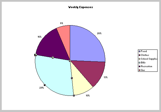
 Select the chart sheet tab to activate the
pie chart.
Select the Pie ring.
Select the chart sheet tab to activate the
pie chart.
Select the Pie ring.
 Select the 29% pie slice.
 Choose Selected Data Point from the
Format menu.
Choose Selected Data Point from the
Format menu.
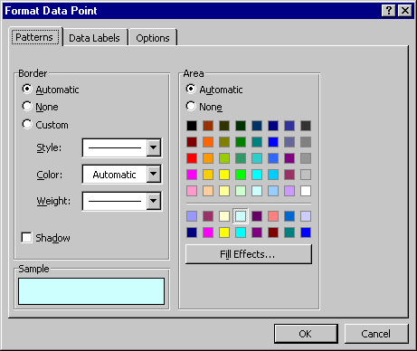 Select the Patterns tab and choose a different
color and pattern for the slice.
Select another pie slice and change its color.
Select the Chart title.
Select the Patterns tab and choose a different
color and pattern for the slice.
Select another pie slice and change its color.
Select the Chart title.
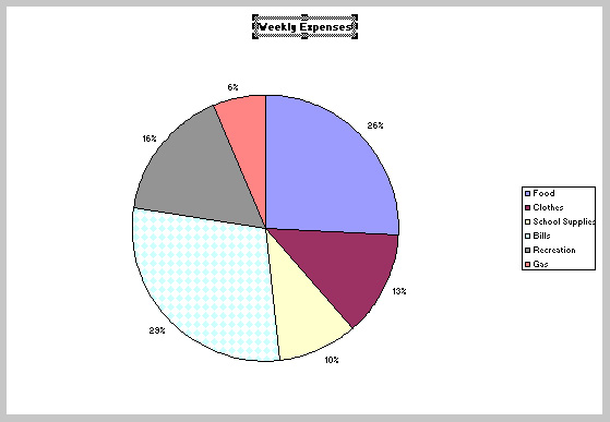 Choose a different color from the
Font Color button
(
Choose a different color from the
Font Color button
( ).
Select the chart.
Save all your changes.
Choose Print Preview from the File
menu.
Click on the Close button.
Choose Page SetUp from the File menu.
Within the Page Setup dialog box
select the Header/Footer tab.
).
Select the chart.
Save all your changes.
Choose Print Preview from the File
menu.
Click on the Close button.
Choose Page SetUp from the File menu.
Within the Page Setup dialog box
select the Header/Footer tab.
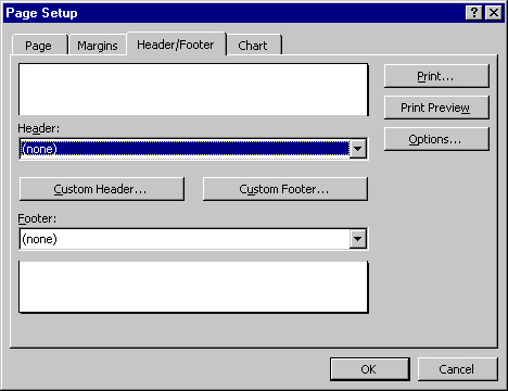 Within the Header/Footer box select none
from the Header and Footer pull-down menus.
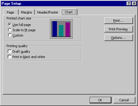
Within the Page Setup dialog box, select
the Chart tab and select the following
setting:
Within the Header/Footer box select none
from the Header and Footer pull-down menus.
Within the Page Setup dialog box, select
the Chart tab and select the following
setting:
 Click on the OK button.
Click on the Print button.
Click on the OK button.
Click on the Print button.
| Next Topic: Column Charts |
|
|